Stability of control Systems

Introduction

As systems become more complex, representing them with differential equations or transfer functions becomes cumbersome. This is even more true if the system has multiple inputs and outputs. This document introduces the state space method which largely alleviates this problem. The state space representation of a system replaces an nth order differential equation with a single first order matrix differential equation. The state space representation of a system is given by two equations :

Note: Bold face characters denote a vector or matrix.The variable x is more commonly used in textbooks and other references than is the variable q when state variables are discussed. The variable q will be used here since we will often use to represent position.

The first equation is called the state equation, the second equation is called the output equation. For an nth order system (i.e., it can be represented by an nth order differential equation) with r inputs and m outputs the size of each of the matrices is as follows:

• q is nx1 (n rows by 1 column); q is called the state vector, it is a function of time
• A is nxn; A is the state matrix, a constant
• B is nxr; B is the input matrix, a constant
• u is rx1; u is the input, a function of time
• C is mxn; C is the output matrix, a constant
• D is mxr; D is the direct transition (or feedthrough) matrix, a constant
• y is mx1; y is the output, a function of time

Note several features:

• The state equation has a single first order derivative of the state vector on the left, and the state vector, q(t), and the input u(t) on the right. There are no derivatives on the right hand side.
• The output equation has the output on the left, and the state vector, q(t), and the input u(t) on the right. There are no derivatives on the right hand side.

For systems with a single input and single output (i.e., most of the systems we will consider) these variables become (with r=1 and m=1):

where

• q is nx1 (n rows by 1 column)
• A is nxn
• B is nx1
• u is 1x1 (i.e., a scalar)
• C is 1xn
• D is 1x1 (i.e, a scalar)
• y is 1x1 (i.e, a scalar)

Advantages of this representation include:

• The notation is very compact. Even large systems can be represented by two simple equations.
• Because all systems are represented by the same notation, it is very easy to develop general techniques to solve these systems.
• Computers easily simulate first order equations.

A Simple Example

Consider an 4th order system represented by a single 4th order differential equation with input x and output y.

We can define 4 new variables, q1 through q4.

but

We can now rewrite the 4th order differential equation as 4 first order equations

This is compactly written in state space format as

with

For this problem a state space representation was easy to find. In many cases (e.g., if there are derivatives on the right side of the differential equation) this problem can be much more difficult. Such cases are explained in the discussion of .

Case 1: Alternate State Space Representation

Another important point is that the state space representation is not unique. As a simple example we could simply reorder the variables from the example above (the new state variables are labeled qnew). This results in a new state space representation

Case 2: Alternate State Space Representations

In the previous case careful examination of the original and modified state space system reveals that they represent the same system. However we can make entirely new state variables by forming linear combination of the original state variables in which this equality is not obvious. Consider the state variable new defined as follows:

In this case the new state space variables are given by:

This new state space system is quite different from the original one, and it is not at all obvious that they represent the same system. (It can be shown that the systems are identical by transforming the state space representation to a transfer function. Techniques for doing so are discussed elsewhere.)

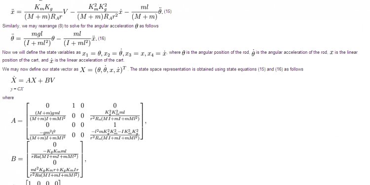
Key Concept: Defining a State Space Representation

A nth order linear physical system can be represented using a state space approach as a single first order matrix differential equation:

The first equation is called the state equation and it has a first order derivative of the state variable(s) on the left, and the state variable(s) and input(s), multiplied by matrices, on the right. The second equation is called the output equation and it has teh output on the left and the state variable(s) and input(s), multiplied by matrices, on the right. No other terms are allowed in the equation. In these equations: