Control Systems transfer function

A Transfer Function is the ratio of the output of a system to the input of a system, in the Laplace domain considering its initial conditions and equilibrium point to be zero. This assumption is relaxed for systems observing transience. If we have an input function of X(s), and an output function Y(s), we define the transfer function H(s) to be:

H(s)=Y(s)X(s){\displaystyle H(s)={Y(s) \over X(s)}}

Readers who have read the Circuit Theory book will recognize the transfer function as being the impedance, admittance, impedance ratio of a voltage divider or the admittance ratio of a current divider.

Impulse Response[edit]

Note:
Time domain variables are generally written with lower-case letters. Laplace-Domain, and other transform domain variables are generally written using upper-case letters.

For comparison, we will consider the time-domain equivalent to the above input/output relationship. In the time domain, we generally denote the input to a system as x(t), and the output of the system as y(t). The relationship between the input and the output is denoted as the impulse response, h(t).

We define the impulse response as being the relationship between the system output to its input. We can use the following equation to define the impulse response:

h(t)=y(t)x(t){\displaystyle h(t)={\frac {y(t)}{x(t)}}}

Impulse Function[edit]

It would be handy at this point to define precisely what an "impulse" is. The Impulse Function, denoted with δ(t) is a special function defined piece-wise as follows:

δ(t)={0, t0undefined, t=00, t0{\displaystyle \delta (t)=\left\{{\begin{matrix}0, &t0\end{matrix}}\right.}

The impulse function is also known as the delta function because it's denoted with the Greek lower-case letter δ. The delta function is typically graphed as an arrow towards infinity, as shown below:

It is drawn as an arrow because it is difficult to show a single point at infinity in any other graphing method. Notice how the arrow only exists at location 0, and does not exist for any other time . The delta function works with regular time shifts just like any other function. For instance, we can graph the function δ(t - N) by shifting the function δ(t) to the right, as such:

An examination of the impulse function will show that it is related to the unit-step function as follows:

δ(t)=du(t)dt{\displaystyle \delta (t)={\frac {du(t)}{dt}}}

and

u(t)=∫δ(t)dt{\displaystyle u(t)=\int \delta (t)dt}

The impulse function is not defined at point t = 0, but the impulse must always satisfy the following condition, or else it is not a true impulse function:

∫−∞∞δ(t)dt=1{\displaystyle \int _{-\infty }^{\infty }\delta (t)dt=1}

The response of a system to an impulse input is called the impulse response. Now, to get the Laplace Transform of the impulse function, we take the derivative of the unit step function, which means we multiply the transform of the unit step function by s:

L[u(t)]=U(s)=1s{\displaystyle {\mathcal {L}}[u(t)]=U(s)={\frac {1}{s}}} L[δ(t)]=sU(s)=ss=1{\displaystyle {\mathcal {L}}[\delta (t)]=sU(s)={\frac {s}{s}}=1}

This result can be verified in the transform tables in .

Step Response[edit]

This operation can be performed using this MATLAB command:

Similar to the impulse response, the step response of a system is the output of the system when a unit step function is used as the input. The step response is a common analysis tool used to determine certain metrics about a system. Typically, when a new system is designed, the step response of the system is the first characteristic of the system to be analyzed.

Convolution[edit]

This operation can be performed using this MATLAB command:

However, the impulse response cannot be used to find the system output from the system input in the same manner as the transfer function. If we have the system input and the impulse response of the system, we can calculate the system output using the convolution operation as such:

y(t)=h(t)∗x(t){\displaystyle y(t)=h(t)*x(t)}

Remember: an asterisk means convolution, not multiplication!

Where " * " (asterisk) denotes the convolution operation. Convolution is a complicated combination of multiplication, integration and time-shifting. We can define the convolution between two functions, a(t) and b(t) as the following:

(a∗b)(t)=(b∗a)(t)=∫−∞∞a(τ)b(t−τ)dτ{\displaystyle (a*b)(t)=(b*a)(t)=\int _{-\infty }^{\infty }a(\tau )b(t-\tau )d\tau }

(The variable τ (Greek tau) is a dummy variable for integration). This operation can be difficult to perform. Therefore, many people prefer to use the Laplace Transform (or another transform) to convert the convolution operation into a multiplication operation, through the Convolution Theorem.

Time-Invariant System Response[edit]

If the system in question is time-invariant, then the general description of the system can be replaced by a convolution integral of the system's impulse response and the system input. We can call this the convolution description of a system, and define it below:

[Convolution Description]

y(t)=x(t)∗h(t)=∫−∞∞x(τ)h(t−τ)dτ{\displaystyle y(t)=x(t)*h(t)=\int _{-\infty }^{\infty }x(\tau )h(t-\tau )d\tau }

Convolution Theorem[edit]

This method of solving for the output of a system is quite tedious, and in fact it can waste a large amount of time if you want to solve a system for a variety of input signals. Luckily, the Laplace transform has a special property, called the Convolution Theorem, that makes the operation of convolution easier:

Convolution Theorem Convolution in the time domain becomes multiplication in the complex Laplace domain. Multiplication in the time domain becomes convolution in the complex Laplace domain.

The Convolution Theorem can be expressed using the following equations:

L[f(t)∗g(t)]=F(s)G(s){\displaystyle {\mathcal {L}}[f(t)*g(t)]=F(s)G(s)} L[f(t)g(t)]=F(s)∗G(s){\displaystyle {\mathcal {L}}[f(t)g(t)]=F(s)*G(s)}

This also serves as a good example of the property of Duality.

Using the Transfer Function[edit]

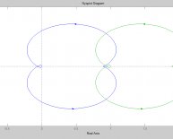
The Transfer Function fully describes a control system. The Order, Type and Frequency response can all be taken from this specific function. Nyquist and Bode plots can be drawn from the open loop Transfer Function. These plots show the stability of the system when the loop is closed. Using the denominator of the transfer function, called the characteristic equation, roots of the system can be derived.

For all these reasons and more, the Transfer function is an important aspect of classical control systems. Let's start out with the definition:

Transfer Function The Transfer function of a system is the relationship of the system's output to its input, represented in the complex Laplace domain.

If the complex Laplace variable is , then we generally denote the transfer function of a system as either G(s) or H(s). If the system input is X(s), and the system output is Y(s), then the transfer function can be defined as such:

H(s)=Y(s)X(s){\displaystyle H(s)={\frac {Y(s)}{X(s)}}}

If we know the input to a given system, and we have the transfer function of the system, we can solve for the system output by multiplying:

[Transfer Function Description]

Y(s)=H(s)X(s){\displaystyle Y(s)=H(s)X(s)}

Example: Impulse Response[edit]

From a Laplace transform table, we know that the Laplace transform of the impulse function, δ(t) is:

L[δ(t)]=1{\displaystyle {\mathcal {L}}[\delta (t)]=1}

So, when we plug this result into our relationship between the input, output, and transfer function, we get:

Y(s)=X(s)H(s){\displaystyle Y(s)=X(s)H(s)} Y(s)=(1)H(s){\displaystyle Y(s)=(1)H(s)} Y(s)=H(s){\displaystyle Y(s)=H(s)}

In other words, the "impulse response" is the output of the system when we input an impulse function.

Example: Step Response[edit]

From the Laplace Transform table, we can also see that the transform of the unit step function, u(t) is given by:

L[u(t)]=1s{\displaystyle {\mathcal {L}}[u(t)]={\frac {1}{s}}}

Plugging that result into our relation for the transfer function gives us:

Y(s)=X(s)H(s){\displaystyle Y(s)=X(s)H(s)} Y(s)=1sH(s){\displaystyle Y(s)={\frac {1}{s}}H(s)} Y(s)=H(s)s{\displaystyle Y(s)={\frac {H(s)}{s}}}

And we can see that the step response is simply the impulse response divided by .

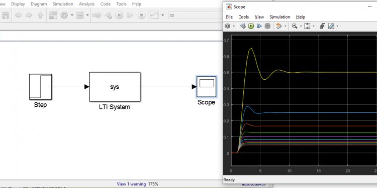
Example: MATLAB Step Response[edit]

Use MATLAB to find the step response of the following transfer function:

F(s)=79s2+916s+1000s(s+10)3{\displaystyle F(s)={\frac {79s^{2}+916s+1000}{s(s+10)^{3}}}}

We can separate out our numerator and denominator polynomials as such:

num = [79 916 1000]; den = [1 30 300 1000 0]; sys = tf(num, den);

Now, we can get our step response from the step function, and plot it for time from 1 to 10 seconds: