Open loop circuit

Graphing the Open Loop Gain of a circuit can be a challenging and time consuming task in PSpice because of a few difficulties with the tool that have been overcome in the latest hotfix (V16.6 S017).

Shortcomings of Previous Versions of PSpice

The first problem was the amount of time that simulating the circuit to get all the data would take. If you want the responses from a wide variety of frequencies and only want to run the simulation once, you can only have one set duration for the simulation which meant that your high frequency signals will have to run a LOT more times than your low frequency signals.

This means that your CPU will be busy crunching a lot of data cycles for your high frequency signals and the higher you go in frequency, the longer the simulation takes (exponentially).

Once you have all the data collected, the second problem is turning the collected time domain information into something that is quickly readable (ie a Bode plot). You could make equations and pull data out and have it plotted but this required a lot of clicks and a fair amount of knowledge.

In the latest version of PSpice, these problems have both been removed to make graphing the open loop gain of a circuit a simple and quick operation.

I’m going to be going over the example FRAEXAMPLE.opj in the C:\Cadence\SPB_16.6\tools\pspice\capture_samples\anasim\fra directory (make sure you have hotfix S017 to see this directory) with just a few slight modifications.

Solving with Middlebrook’s Method

By using ‘Middlebrook’s Method’ on linear, closed loop systems, we are able to determine the open loop response. This is done by injecting small test signals in a point of the circuit where a low impedance drives a high impedance. A point like this can usually be found in a SMPS design where the power supply drives an amplifier input. At this point in the feedback loop, the current gain should be zero and the voltage gain can be used as the loop gain.

Using a Text Block as a Simulation Profile

The first new feature in PSpice is the ability to use a text block on your schematic as your simulation profile. This may seem like a step backwards back to the days of hand entering SPICE netlists but in this case, it gives us the flexibility to add a formula into the total simulation time field.

Taking a look at the simulation profile that’s been set up as a text block in the FRAEXAMPLE file, we see:

@PSpice:
.TRAN 0 {5/Freq}
.STEP DEC PARAM FREQ 0.1 1MEG 7
.PROBE64 P(FREQ)
.options MINSIMPTS = 1000

Where the:

@PSpice: - means that the tool should look at this text block for the profile information

.TRAN 0 {5/Freq} – means that we’re doing a transient simulation with no specific minimum step size (the 0) and a total simulation time of 5/Freq which equates to 5 periods at whatever frequency we’ll be running in a particular sweep case (see next item).

The ability to put an equation in the value for total simulation time means that it will take just as much CPU time to run the low frequency signals as it does for the high frequency signals because it’s doing just 5 periods regardless of frequency. This is the first part of solving our first problem of taking too much simulation time.

In the FRAEXAMPLE, it would take about 30 minutes of CPU time and have an extremely large .DAT file without this vs. about 5 seconds to run the complete simulation using this variable total simulation time and a tiny .DAT file that’s consequently easy to manage.

Normally the Minimum Step Size is used to accomplish this but in this case, with the frequency constantly changing, that’s not possible without again increasing the CPU simulation time for the low frequency signals that have to take a lot of sample points to keep up the resolution on the high frequency signals. This is the second part to solving the simulation taking too much time.

Simulating and Viewing the Results

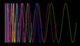
When the simulation is run, the results look pretty meaningless and messy but there is a lot of important details stored in there. First, you can see that the simulation end point changes with each of the traces, this is what saves us a lot of simulation time.

Let’s take a look at the data from a single simulation sweep, the first simulation run (FREQ=0.1Hz). You can do this by adding the traces you want to see with an @1 sign afterwards which indicates that you just want the results from the first simulation run.

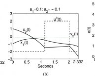
We can verify from this is that there are only 5 periods of data, next we want to understand the relationship between V(A) and V(B). V(B) appears to be out of phase by 180 degrees with respect to V(A) at 0.1Hz.

Dividing V(A) by V(B) tells us that it’s 49, 751 times larger than V(B) which is the amplification at 0.1Hz.

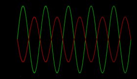
To collect another sample data point, let’s take a look at the last (50th) simulation run (FREQ=1 MHz) to see what the relationship is there:

V(B) appears to be lagging by 90 degrees with respect to V(A) at 1 MHz. Dividing V(A) by V(B) tells us that it’s 4.97 times larger than V(B) which is the amplification at 1 MHz.

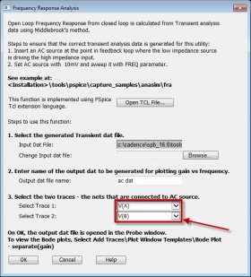
Frequency Response Analysis (FRA)