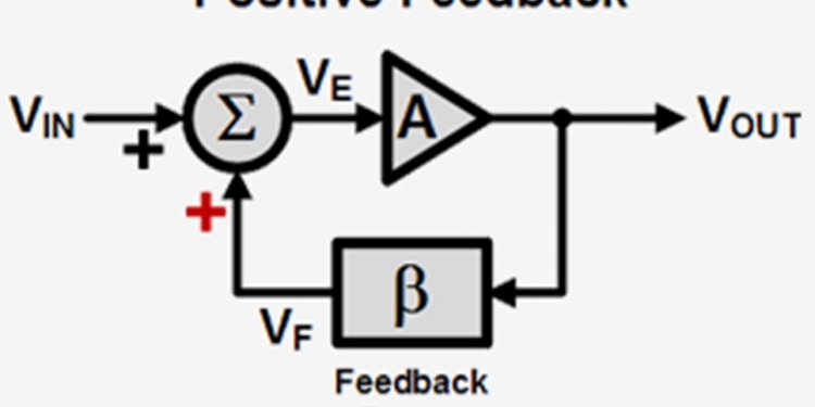
Positive feedback block diagram

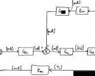
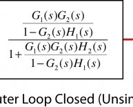
where state variables M, P and T stand for the mRNA, permease and internal TMG concentration, respectively. The inputs T e and G e represent the external TMG and external glucose concentration, respectively. γ i with i A f M ; P ; T g represents the loss constants for M, P, and T ; γ i represents the composition of the active degradation, γ i, and the dilution due to growth rate, μ i, i.e., γ i 1⁄4 γ i þ μ i . α i with i A f M ; P ; T g denotes the production constants of the gene products. f M ; T ð T Þ and f M ; G e ð G e Þ express the positive effect of the internal TMG and the negative effect of external glucose on the synthesis of mRNA, respectively. Similarly, f T ; T e ð T e Þ and f T ; G e ð G e Þ express the positive effect of external TMG and negative effect of external glucose on TMG uptake into the cell, respectively. Here, f M ; G e ð G e Þ and f ð G Þ are decreasing functions of external glucose; the former describes catabolite repression, while the latter describes inducer exclusion. Regarding the TMG-induced lac operon model, the temporal change in mRNA concentration is de fi ned in (1) as the difference between the production depending on the internal TMG concentration under the catabolite repression effect of external glucose and the losses due to active degradation and growth. Equation (2) accounts for the change in permease concentration in terms of synthesized permease and losses. Similarly, the change in the internal TMG concentration is expressed in (3), where an increase in TMG is due to the import of the external TMG under the reduction effect of inducer exclusion, and a decrease is due to its degradation and dilution. Assuming the production of mRNA under TMG as an allosteric interaction similar to that of allolactose, f M ; T ð T Þ can be calculated using the following modi fi ed Hill function [39]: f ð T Þ 1⁄4 1 þ K 1 T n ð 4 Þ where n is the number of TMG required to inactivate a repressor protein, K 1 is the equilibrium constant of the TMG – repressor protein interaction, and 1 = K is the basal level of mRNA transcription in E. coli . For the inhibition of repressor protein, at least two TMG molecules must bind the repressor. Thus, n equals 2 in the analyses throughout this study. The root locus method is a well-known classical method in control area to determine the changes of the location of closed- loop system poles as a function of a model parameter. The usual concern in control applications employing the root locus method is to identify the range of a controller parameter ensuring a desired behavior of the closed-loop system such as Lyapunov (asymptotic) stability which is obtained for the closed-loop poles all in the open left half-plane. As described in Subsection 3.1, the poles of the Laplace domain (closed-loop) transfer function are indeed the roots to the characteristic equation which is a rational function of s complex variable. So, studying the positions of the poles in the complex plane is equivalent to determine the positions of the roots to a polynomial equation. This classical method of root locus is actually valid for any kind of polynomial equations with real-valued coef fi cients. The proposed application of the root locus method for the bistability analysis of lac operon relies on the following facts: (i) ODE models derived from mass action kinetics with Michaelis – Menten or Hill approach have state equation forms with rational right hand sides, so their rational equilibrium equations can be rearranged as polynomial equations. (ii) For a deterministic dynamical system de fi ned by ODEs, in particular lac operon model given by (1) – (3), a bistable behavior requires triple equilibria which are actually the real roots to the equilibrium equation, exactly two of which are asymptotically stable in the sense of Lyapunov [37]. So, for the polynomial equilibrium equation case, the range of a speci fi c model parameter ensuring three real equilibria can be found by applying the classical root locus to this equilibrium equation. To make the paper self-contained, the classical root locus method is brie fl y described in Subsection 3.1. Subsection 3.2 demonstrates the applicability of the root locus method for studying the change of the equilibrium point(s) of gene regulatory networks on a simple synthetic model representing the production and degradation of a biological molecule. Subsection 3.3 which considers a rather complicated production – degradation model available in the literature is devoted to show that the root locus method is by no means restricted to equilibrium equations of three or less degree as appeared in the bistability analysis of lac operon model presented in Section 4 but valid for the equilibrium equations of arbitrary degree. To describe the root locus method, let consider a linear time- invariant single-input single-output control system depicted in Fig. 2 where G c ( s ), G p ( s ) and H ( s ) are the Laplace domain transfer function of the controller, plant and sensor, respectively. The closed-loop transfer function is given as